Introduction

Welcome to my exploration of Generative Adversarial Networks (GANs), where artificial intelligence meets creativity. I want to take you on a journey into the inner workings of GANs and show you their remarkable ability to generate stunningly realistic handwritten digit images.

GANs represent a fundamental shift in machine learning. Rather than learning to classify or predict, they learn to create. This generative capability opens new frontiers in artificial intelligence, from data augmentation and content generation to artistic expression and beyond.

From data preparation and model design to training and evaluation, I'll uncover the mechanics behind GANs and reveal the incredible potential these generative models hold. My implementation focuses on the MNIST dataset, providing a clear demonstration of how adversarial training enables neural networks to generate realistic synthetic data.

Background: Understanding GANs

The Adversarial Framework

Generative Adversarial Networks consist of two neural networks engaged in a competitive game:

• Generator: Creates synthetic data from random noise
• Discriminator: Distinguishes real data from generated samples

This adversarial process drives both networks to improve. The generator learns to create increasingly realistic samples, while the discriminator becomes better at detecting fakes. At equilibrium, the generator produces samples indistinguishable from real data.

The MNIST Dataset

I'm using the MNIST dataset of handwritten digits:

• Training samples: 60,000 grayscale images
• Image dimensions: 28×28 pixels
• Classes: Digits 0-9
• Format: Pixel values normalized to [0, 1]

This dataset provides an ideal testbed for GAN development. It offers sufficient complexity while remaining computationally tractable.

Data Preparation

Loading and Transforming Data

The first critical step involves preparing our MNIST dataset for GAN training. We implement a get_dl function to handle data transformation and loading:

Data Processing Pipeline

This method accomplishes several critical tasks:

1. Data Transformation: We use transforms.Compose to create a transformation pipeline. The transforms.ToTensor() operation converts raw image data into PyTorch tensors, essential for neural network processing.

2. Data Download and Transformation: The MNIST dataset is downloaded with training and testing datasets saved in separate directories. We apply transformations to convert these datasets into tensors.

3. Data Loading: We utilize PyTorch's DataLoader class for efficient batch processing. Key parameters include:

   • batch_size: Number of samples per batch
   • shuffle=False: Maintains data order within batches
   • drop_last=True: Drops incomplete final batches to maintain consistent batch sizes

4. Return Values: The function returns train_loader and test_loader objects for use during training and evaluation.

With our data pipeline established, we're equipped to train our GAN to generate realistic handwritten digits.

Model Architecture

Generator Network Design

The generator network transforms random noise into synthetic images. Our Generator class implements this transformation:

Generator Architecture Details

Initialization: The constructor accepts two parameters:

• batch_size: Number of samples generated per batch
• input_dim: Dimensionality of the input noise vector (latent space)

Network Layers:

• self.fc1: First fully connected layer mapping input_dim → 128 dimensions, followed by Leaky ReLU activation
• self.fc2: Second fully connected layer mapping 128 → 784 (28×28) dimensions, followed by Tanh activation

Forward Propagation: The forward pass:

1. Transforms input noise through fc1 with Leaky ReLU activation
2. Maps to image space through fc2 with Tanh activation (output range [-1, 1])
3. Reshapes output to match MNIST image dimensions [batch_size, 1, 28, 28]

The generator progressively learns to map random noise to realistic digit images through adversarial training.

Discriminator Network Design

The discriminator evaluates whether images are real or generated. Our Discriminator class implements this binary classification:

Discriminator Architecture Details

Initialization: The constructor accepts batch_size to process samples in batches.

Network Layers:

• self.fc1: First fully connected layer mapping 784 (flattened 28×28 image) → 128 dimensions with Leaky ReLU activation
• self.fc2: Second fully connected layer mapping 128 → 1 dimension with Sigmoid activation (output range [0, 1])

Forward Propagation: The forward pass:

1. Flattens input images to 1D vectors
2. Processes through fc1 with Leaky ReLU activation
3. Maps to scalar confidence score through fc2 with Sigmoid activation
4. Reshapes output to single scalar per sample

The Sigmoid output represents the discriminator's confidence that the input is real (values near 1) versus fake (values near 0).

Training Procedure

The Training Loop

The train_model function orchestrates the adversarial training process:

Training Dynamics

The training procedure implements the adversarial game:

Device Selection: Automatically detects and utilizes GPU acceleration if available.

Discriminator Training:

1. Evaluate real images and compute loss against real labels
2. Generate fake images from random noise
3. Evaluate fake images (detached from generator graph) and compute loss against fake labels
4. Backpropagate combined loss and update discriminator parameters

Generator Training:

1. Generate fake images from random noise
2. Pass through discriminator (with gradient flow)
3. Compute loss against real labels (fool the discriminator)
4. Backpropagate and update generator parameters

Key Insight: The generator is trained to maximize discriminator error by labeling fake images as real, while the discriminator learns to correctly classify both real and fake samples.

Experimental Setup

Configuration and Initialization

We establish the complete training configuration:

Hyperparameter Selection

Reproducibility: Fixed random seed ensures consistent results across runs.

Training Parameters:

• Batch size: 128 samples
• Epochs: 5 iterations through dataset
• Latent dimension: 100-dimensional noise vectors

Optimization:

• Algorithm: Adam optimizer for both networks
• Learning rate: 0.001
• Weight decay: 1e-05 for regularization
• Loss function: Binary cross-entropy

These hyperparameters balance training stability with convergence speed, crucial for successful GAN training.

Training Results

The training process demonstrates progressive improvement:

Epoch 1/5
Discriminator Loss: 428.8399
Generator Loss: 752.0623

Epoch 2/5
Discriminator Loss: 667.7617
Generator Loss: 519.8400

Epoch 3/5
Discriminator Loss: 662.0597
Generator Loss: 413.3630

Epoch 4/5
Discriminator Loss: 593.1331
Generator Loss: 427.6587

Epoch 5/5
Discriminator Loss: 597.1973
Generator Loss: 450.6230

The loss trajectories indicate successful adversarial training, with both networks adapting to each other's improvements.

Results and Visualization

Generating Synthetic Digits

We visualize the generator's output using the following code:

Generated Samples

The result displays 50 synthetic handwritten digits generated by our trained GAN:

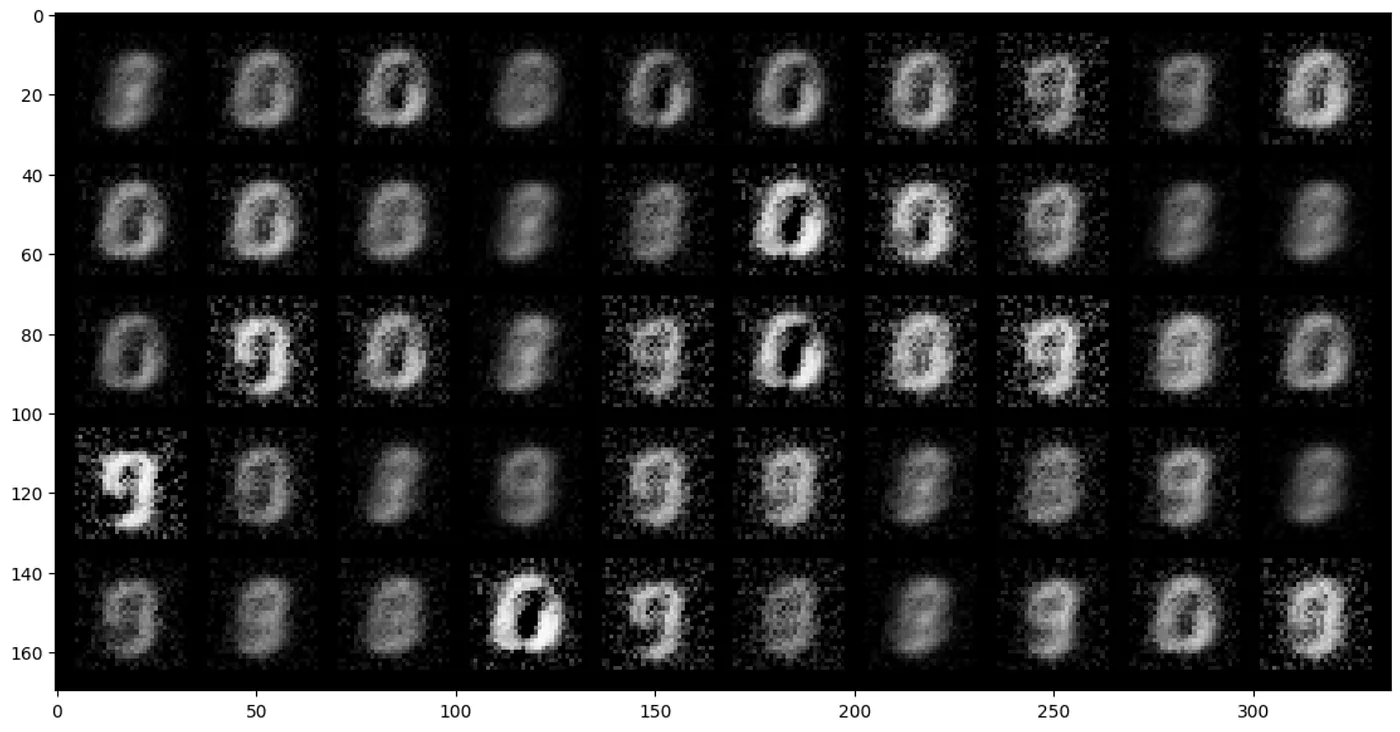
Each image represents the generator's learned understanding of handwritten digit structure. The quality and diversity of these samples demonstrate successful adversarial training.

Discussion

Training Dynamics and Convergence

Our implementation demonstrates several key aspects of GAN training:

Loss Behavior: The discriminator and generator losses fluctuate throughout training, reflecting the adversarial dynamics. This instability is characteristic of GANs and indicates both networks are actively learning.

Quality Progression: Generated samples improve significantly from random noise to recognizable digits, validating the adversarial training framework.

Architectural Choices: The simple fully-connected architecture proves sufficient for MNIST, though more complex datasets would benefit from convolutional architectures.

Challenges and Considerations

Mode Collapse: GANs can suffer from mode collapse where the generator produces limited variety. Our results show reasonable diversity across digit classes.

Training Stability: Balancing discriminator and generator learning rates is crucial. Too strong a discriminator prevents generator learning; too weak allows poor quality outputs.

Evaluation Metrics: Unlike supervised learning, GANs lack clear objective metrics. Visual inspection and downstream task performance provide the primary evaluation methods.

Conclusion

I've shown you how to implement and train Generative Adversarial Networks for handwritten digit generation. Through systematic exploration of data preparation, model architecture, and training procedures, I've demonstrated how adversarial learning enables neural networks to generate realistic synthetic images.

GANs represent a paradigm shift in artificial intelligence. They move beyond classification and prediction to genuine creation. From data augmentation and content generation to artistic expression, GANs demonstrate the creative potential of machine learning.

The adversarial framework (two networks competing to improve) provides a powerful mechanism for unsupervised learning. As the field evolves, GANs continue pushing the boundaries of what's possible at the intersection of technology and imagination.

The journey of GANs has only begun. Future developments in architecture design, training stability, and application domains promise even more remarkable creations. The extraordinary is becoming reality, one generated pixel at a time.